Visual interface
Gravity.jl includes extensions to visualize the results of a strong lensing modeling. Currently, this functionality is based on the Aladin-lite tool, on the Makie ecosystem, or on the XPA Messaging System for SAOImage DS9.
The visual interface is structured on several layers.
At the highest layer, there are several plotting routines that always takes a fixed set of arguments: an optional backend (for example, :Makie), a gravity-model, and the set of parameters used for the plot. Optionally, some functions associated to a redshift, take the source redshift as an additional (optional) argument (if missing, the source with the highest redshift present in the model is used). All the routines at the highest level ultimately call intermediate-layer routines and pass them all optional keywords eventually present.
At the intermediate layer, there are similar plotting routines. These accept a variety of arguments and, for some backends, also need additional information (for example, the :XPA backend typically requires the model WCS). They also process the keywords that controls the plotting styles: color, line thickness, line styles... Since different backend could have different capabilities, the keyword parameters accepted by the intermediate layer is not completely backend-independent. However, an effort is done to make the plots as similar as possible among the various backends.
At the lower layer, there are a set of very specific routines. These are not exported and are hidden in the various extensions and are not documented here. They take care of all the peculiar steps necessary to make plots in each specific backend.
Backends
Gravity.jl consider two hierarchical backend levels. Major backends are associated to extensions, such as Aladin (always available), Makie (loaded, for example, with commands such as using CairoMakie or using GLMakie) or XPA (loaded with using XPA, to be used with SAOImage DS9). Minor backends should be understood as windows of a given plotting package: for example, one might have two SAOImage DS9 viewers opens, and it might be necessary to choose the one to use for future operations.
Major backends can be specified in each of the following commands using an associated symbol, currently :Aladin, :Makie, or :DS9. If unspecified, the latest loaded extension is used (or :Aladin if no extension is loaded).
Minor backend can be specified using a backend-specific syntax. In particular, for Makie one needs to provide a Makie.Axis object, while for XPA/DS9 one needs to provide a XPA.AccessPoint. The minor backends associated to each major backend can be retrieved with the routine Gravity.get_plotting_backends. It is unnecessary to specify the minor backend if a major backend has a single minor backend (for example, a single SAOImage DS9 window is open).
More simply, one can select the future (major and minor) plotting backend with a simple interface based on the Gravity.set_plotting_backend routine.
Gravity.set_plotting_backend — Function
set_plotting_backend([backend::Symbol]; silent=false)
set_plotting_backend(backend::Val, minor_backend; silent=false)
Set the default plotting backend.
backend, if provided, must be a symbol or a string representing a valid backend (currently, :Makie or :DS9). If not provided, and if more than one backend are loaded, the user is presented with a simple terminal interface to select the backend.
The version with two arguments allows one to specify not only the backend, but also the minor_backend. This function should be implemented by the extension.
Note that in order to enable plotting backends one needs to load the corresponding package as in the in two examples below:
julia> using CairoMakie

julia> using XPATo use of the XPA extension it is necessarly to have SAOImage DS9 opened with a correctly WCS-aligned image. Make sure also that the wcs_origin special parameter or the WCS section of the configuration file have set consistently with the displayed image.
Gravity.current_backend — Function
current_backend([backend::Val])Return the currently default plotting backend as a symbol.
This function works at two levels. If no argument is provided, it returns the major backend type (for example, :DS9 for SAOImage DS9). If, instead, a backend as a Val is given as argument as in current_backend(Val(:DS9)), this function returns the minor backend type (in this case, the DS9 access point linked to a specific SAOImage DS9 window). The latter operation is demanded to each extension.
Gravity.get_plotting_backends — Function
get_plotting_backends()
get_plotting_backends(backend)
Return the major backends or minor backends provided by the major backend.
This is used to dynamically obtain the major and minor backends available. Multiple minor backends can be present when a major backend is able to interact with multiple windows, as in the case of SAOImage DS9.
Filtering
Many plotting routines accepts a filter keyword which can be used to select a subset of the corresponding objects. For example, plotimages! displays the images included in a gravitational lensing model on the default backend. Optionally, one can display just a subset of the images by specifying, with the filter keyword, one of the following:
- A glob pattern as a string (for example,
"*_XPixelated_*") - A regular expression (for example,
r"^sources_1_") - A list (or tuple, or set) of strings for exact matches
- A function that takes an image name as inputs and returns
trueorfalse
Common plot attributes
Most routines described below use a standard set of plot attributes: these will be converted into the appropriate calls by each backend.
color: the line of symbol color, often entered as symbol mnemonic (such as:red)linewidth: the width of the line (default: 1)linestyle: the drawing style of the line (default::solid); other allowed values depend on the backend (for example: Makie allows line styles such as:dash,:dot,:dashdot,:dashdotdot...)symbol: the symbol used for dot-like objects: can be:+(cross),:x,:*,:box,:diamond,:o.scale: the size of the symbol for dot-like object in some backend-specific unit (default: 1)font: the font name as a stringfontsize: the size of the font in points
Backend-specific notes
Aladin backend
The Aladin-lite backend is always available, as it does not require any external package to work. When a plot in this backend is requested, for example with the command plotmodel(model, best_fit), Gravity.jl creates a temporary directory with the necessary code (mostly based on JavaScript). The index.html file of this directory is then loaded with the default system browser. If necessary, one can retrieve the path of the directory used with Gravity.aladin.path.
Note that, due to some limitations of Aladin-lite, this backend cannot show raster images (such as extended images or predictions).
Aladin also has a special behavior when showing background images with `plotbackground!. In particular, if a model background image has been specified in the configuration file using the background special parameter, and the image is associated with an URL, the URL is used; otherwise, or in case a local image directly used with this command, the image is uploaded to a temporary server (currently, https://tempfile.org/) and the associated URL is used. Note that the server stores the image for 24 hours, so that Gravity.jl will re-upload it if necessary after this time span.
XPA backend
The XPA backend understands two specific attributes:
output: if set to a string, the plotting routine will save the region file normally sent to DS9 to a text file with the provided name; alternatively, if set tostdout(or to any other IO object), the region file will be displayed. The default is to haveoutput=nothing, indicating the normal behavior (commands sent to DS9).keep: DS9 bang (!) plotting commands (such asplotlenses!) generally erase the corresponding objects (in the example, all displayed lenses), unlesskeep=true.
Additionally, the XPA background has a special behavior for the plotbackground function: when called, it will create a new frame and show there the background image (note that the frame created will be an RGB frame if the background requires so). This is in contrast to all other XPA plotting routines, which (independently from the absence of the ! at the end) will never create a new frame.
Note, also, that plotmodel and plotmodel! for the XPA background will not call plotbackground.
Highest-level routines
As mentioned above, all the following routines takes standards arguments: an optional major backend as a symbol or alternatively an optional minor-backend (for example, a Makie.Axis object or an XPA.AccessPoint object) a gravity-model, and the set of parameters used for the plot, optionally followed by a redshift.
Gravity.plotlenses! — Method
plotlenses[!]([backend], model, pars; kw...)Display the lenses using the given backend or the last backend.
The lenses have a size which is proportional to their Einstein radius. Undercritical lenses, having therefore a vanishing Einstein radius, will have a size proportional to the minsize keyword. One can use a negative value for the keyword redshift to avoid the situation where several lenses are shown as undercritical.
Keywords
filter: if specified, can be used to display a subset of lenses (can be a string interpreted as a globbing pattern, a regular expression, a list, or a function of the lens names)fill: the color used to fill the lenses as a float (indicating a transparency value, by default 0.1) or a tuple (color, transparency)scale: a positive number used to rescale all Einstein radii (default: 0.25)minsize: the minimum size a lens can have, used to display undercritical lenses (default: 0.1)redshift: this is passed directly to the functionGravity.einsteinradiusand used to compute the size of each lens; therefore, if positive, this is taken as the redshift of the source, while if negative is taken to be -Dₗₛ/Dₛ; the default is -1, corresponding to Dₗₛ/Dₛ = 1, one can use for exampleredshift=-2to enlarge the size of lenses (and display undercritical lenses as critical)format: The format to use for labels: "%l" is replaced with the lens name and "%z" with the lens redshift (default: "%l" if plotting up to 5 lenses, "" otherwise)
The standard keywords color, linewidth, linestyle, font, fontsize are recognized.
Gravity.plotimages! — Method
plotimages[!]([backend], model, pars; kw...)Plot the images present in the model.
Point-like images are shown as simple geometric figures; extended images are shown as iso-luminosity contour plots or as heatmaps, depending on the value of the levels keyword (see plotmass! for common display parameters for extended images).
Keywords
filter: if specified, can be used to display a subset of images (can be a string interpreted as a globbing pattern, a regular expression, a list, or a function of the image names)format: the format to use for the image names: can use "%s" and "%i" to represent, respectively, the source and image name, "%z" the source redshift, "%m" the image magnitude, and "%t" the image time delay (default:"%s.%i"if there are several sources; "%i" otherwise)scale: a positive number used to rescale all uncertainties (default: 0, i.e. no uncertainties are shown)minsize: the minimum size an uncertainty can have (default: 0.1)levels: ifnothing, extended images are shown as heatmaps, otherwise as contour plots
The standard keywords color (default: :magenta), shape (default: :ellipse), size, linewidth, linestyle, font, fontsize are recognized.
Gravity.plotpredictions! — Method
plotpredictions[!]([backend], model, pars; kw...)Plot the images predicted by model from the given parameters.
Point-like predicted images are shown as simple geometric figures; extended images are shown as iso-luminosity contour plots or as heatmaps, depending on the value of the levels keyword (see plotmass! for common display parameters for extended predictions).
Keywords
filter: if specified, can be used to display a subset of predictions (can be a string interpreted as a globbing pattern, a regular expression, a list, or a function of the image names)format: the format to use for the image names: can use "%s" and "%i" to represent, respectively, the source and image name, "%z" the source redshift, "%m" the image magnitude, and "%t" the image time delay (default: "", i.e. no text is shown)scale: a positive number used to rescale all uncertainties (default: 0, i.e. no uncertainties are shown)minsize: the minimum size an uncertainty can have (default: 0.1)levels: ifnothing, extended images are shown as heatmaps, otherwise as contour plots
The standard keywords color (default: :green), shape (default: :x), size, linewidth, linestyle, font, fontsize are recognized.
Gravity.plotsources! — Method
plotsources[!]([backend], model, pars; kw...)Plot the sources predicted by model from the given parameters.
Keywords
filter: if specified, can be used to display a subset of sources (can be a string interpreted as a globbing pattern, a regular expression, a list, or a function of the source names)format: the format to use for the image names: can use "%s" and "%i" to represent, respectively, the source and image name, "%z" the source redshift, "%m" the source magnitude, and "%t" the source time delay (default: "", i.e. no text is shown)scale: a positive number used to rescale all uncertainties (default: 0, i.e. no uncertainties are shown)minsize: the minimum size an uncertainty can have (default: 0.1)
The standard keywords color (default: :orange), shape (default: :x), size, linewidth, linestyle, font, fontsize are recognized.
Gravity.plotcounterimages — Method
plotcounterimages[!]([backend,] model, pars, z [, x₁, x₂...]; kw...)
plotcounterimages[!]([backend,] model, chain, z [, x₁, x₂...]; kw...)
Display the counter-images associated to one or more images.
This function compute the counter-image position(s) associated to one or more images. For interactive backends, this function can also let the user to choose the image position on the screen. Otherwise, each of the xᵢ must be either a multivariate distribution, or a tuple with the coordinates of the image position. The counter-images are found using Gravity.counterimages.
The parameters z can be a single positive value (the sounrce redshift), or also a vector (or range): in that case, a set of counter-images are displayed corresponding to the different redshifts. In this case, format by default is "%z", so that the source redshift is displayed.
Alternatively, the second argument can be an MCMCChains.Chains object, in which case the counter-images are computed for random samples of the chain (by default, 10 samples are used; this can be changed using the nsamples keyword).
Keywords
scale: a positive number used to rescale all uncertainties (default: 0, i.e. no uncertainties are shown)minsize: the minimum size an uncertainty can have (default: 0.1)format: the format to use for the image names, where "%m" will be replaced by the image magnitude and "%t" by the image time delay (default: "", i.e. no text is shown)nsamples: when using anMCMCChains.Chainsobject, the number of random samples to use (default: 10)
The standard keywords color (default: :orange), shape (default: :x), size, linewidth, linestyle, font, fontsize are recognized.
Other keywords (grid=:auto, cricticalcurves=3, images=3, lenses=3 are passed to Gravity.counterimages.
Gravity.plotcriticallines! — Function
plotcriticallines[!]([backend], model, pars [, z]; kw...)
plotcriticallines[!]([backend], model, chain [, z]; kw...)
Display the critical lines associated to the model.
Lines are displayed at the redshift(s) z (which can be a single value or a vector of reals); by default z is set to the redshift of the most distant source.
The second argument can also be an MCMCChains.Chains object, in which case the critical lines are computed for random samples of the chain (by default, 10 samples are used; this can be changed using the nsamples keyword).
Keywords
grid: AGravity.MaskedGridor:auto(the default), to have the grid automatically computed usingGravity.lensing_arealevels: a positive integer the number of contours to show, or an array with the exact values of the levels to display (default: 7)refinements: the refinements to compute around the contours (default: 3)nsamples: when using anMCMCChains.Chainsobject, the number of random samples to use (default: 10)
The standard keywords color (default: :cyan), linewidth, and linestyle are recognized.
Gravity.plotcaustics! — Function
plotcaustics[!]([backend,] model, pars [, z]; kw...)
plotcaustics[!]([backend,] model, chain [, z]; kw...)
Display the caustics associated to the model.
Lines are displayed at the redshift(s) z (which can be a single value or a vector of reals); by default z is set to the redshift of the most distant source.
The second argument can also be an MCMCChains.Chains object, in which case the caustics are computed for random samples of the chain (by default, 10 samples are used; this can be changed using the nsamples keyword).
Keywords
grid: AGravity.MaskedGridor:auto(the default), to have the grid automatically computed usingGravity.lensing_arealevels: a positive integer the number of contours to show, or an array with the exact values of the levels to display (default: 7)refinements: the refinements to compute around the contours (default: 3)nsamples: when using anMCMCChains.Chainsobject, the number of random samples to use (default: 10)
The standard keywords color (default: :pink), linewidth, and linestyle are recognized.
Gravity.plotmass! — Function
plotmass[!]([backend,] model, pars; kw...)Display the mass map for a model.
This function displays the mass map associated to model with the given parameters. The mass map, by default, is displayed as a contour map, unless levels=nothing, in which case the display is a heatmap.
For countours display (default), the function is evaluated at the corners of grid (which must be a Gravity.MaskedGrid), and refinements are possibly computed.
For heatmap display (levels=nothing), the function is evaluate at the centers of grid (which must be a Gravity.BasicGrid).
Keywords
grid: AGravity.MaskedGrid(for contour plots), aGravity.BasicGrid(for heatmap plots) or:auto(the default), to have the grid automatically computed usingGravity.lensing_arealevels: a positive integer the number of contours to show, or an array with the exact values of the levels to display (default: 7); uselevels=nothingto display the mass as a heatmaprefinements: the refinements to compute around the contours (default: 3)transfer: The result offunis passed totransferto increase the dynamic range (default::sqrt)
The standard keywords color, linewidth, and linestyle are recognized.
Gravity.plotmagnification! — Function
plotmagnification[!]([backend,] model, pars [, z]; kw...)Display the magnification for a model at redshift z.
This function displays the magnification associated to model with the given parameters, at redshift z; if the redshift is not provided, the redshift of the most distant source is used. The magnification map, by default, is displayed as a contour map, unless levels=nothing, in which case the display is a heatmap.
For countours display (default), the function is evaluated at the corners of grid (which must be a Gravity.MaskedGrid), and refinements are possibly computed.
For heatmap display (levels=nothing), the function is evaluate at the centers of grid (which must be a Gravity.BasicGrid).
Keywords
grid: AGravity.MaskedGrid(for contour plots), aGravity.BasicGrid(for heatmap plots) or:auto(the default), to have the grid automatically computed usingGravity.lensing_arealevels: a positive integer the number of contours to show, or an array with the exact values of the levels to display (default: 7); uselevels=nothingto display the mass as a heatmaprefinements: the refinements to compute around the contours (default: 3)transfer: The result offunis passed totransferto increase the dynamic range (default::sqrt)
The standard keywords color, linewidth, and linestyle are recognized.
Gravity.plotbackground! — Function
plotbackground[!]([backend], model; kw...)
plotbackground[!]([backend], image [, wcs]; wcs=global_wcs, kw...)
Plot the background image associated to model (if any).
Alternatively, one can provide directly an image, as a filename (as a PNG, JPEG, JPEG2000, TIFF, or FITS) or as an array. If the optional wcs argument is provided, it is used to display the image with the correct astrometry; if not provided, the WCS is extracted from the FITS header or from the AVM tags (present in PNG, JPEG, JPEG2000, and TIFF files).
Gravity.plotgrid! — Method
plotgrid[!]([backend], model, pars; kw...)Plot the lens-inversion grid associated to model (if any).
See above for the accepted keywords.
Gravity.plotmodel — Function
plotmodel[!]([backend,] model, pars [, z]; kw...)
plotmodel[!]([backend,] model, chain [, z]; kw...)
Make a full plot of a gravitational model.
model must be a GravityModel (loaded with gravitymodel), and pars must be the associated free parameters.
The display is done using the specific backend, which can be a specific objects (for example, a Makie.Axis) or a symbol referring to a backend (for example, :Makie). If not specified, the latest loaded graphic backend is used.
If the second argument is an MCMCChains.Chains object, the model is plotted for the best-fit parameters found in the chain. If z is provided, it is used as the source redshift for the critical lines and caustics display; otherwise, the redshift of the most distant source is used.
Keyword parameters
Most keyword parameters accepted are used to specify the objects to plot and the corresponding style:
lenses: control the display of the lenses usingplotlenses!;true_lenses: control the display of the lenses at their true position usingplotlenses!: it is equivalent tolenseswhenlens_lenses = false;images: control the display of the observed images usingplotimages!;predictions: control the display of the predicted images, also usingplotimages!(with different default styles);sources: control the display of the sources usingplotimages!;criticallines: control the display of the critical lines usingplotcriticallines!;caustics: control the display of the caustics usingplotcaustics!(disabled by default);grid: control the display of the model grid (if present) usingplotgrid!(disabled by default).mass: control the display of the mass distribution usingplotmass!(disabled by default);truemass: control the display of the true mass distribution usingplottruemass!(disabled by default);magnification: control the display of the magnification contours usingplotmagnification!(disabled by default);
All these keywords arguments can be of different forms:
true: the corresponding object will be shown with the default style;false: the corresponding object will not be shown;- a named tuple or dictionary: the corresponding object will be shown with a style updated accordingly (for example,
lenses=(; color=:yellow)will display the lenses in yellow); note that the specific style parameters are backend-dependent.
The default is to display the lenses (lenses=true), observed images (images=true), predicted images (predictions=true), and the critical lines (critical_lines=true).
Specific backends can support other parameters. In particular, Makie also recognizes limits, which is directly passed to the Axis call.
True mass distribution
For multi-plane lenses, it might be interesting to display the true mass distribution, i.e. the lens configuration one would observe in absence of lensing. This can be carried out using the two routines described below, which have identical syntax as the corresponding standard routines discussed above.
As an example, the following figure reports the data shown in SAOImage DS9 with the following commands:
julia> model = gravitymodel("examples/HE0435-1123/HE0435-1123mag.yml")
Main.GravityModel

julia> chain = runmodel(model);

julia> x = bestlp(chain)[2]
6-element Vector{Float64}:
 254.15048135481314
   0.2469213324203622
   0.7707409420002984
   0.02351167383066497
  -0.06197635987278063
 201.50423747216183
followed by
julia> plotmodel(model, x; lenses=false, criticallines=false, mass=true, truemass=true)The same result can be obtained with the sequence of commands
julia> plotimages(model, x)

julia> plotpredictions!(model, x)

julia> plotmass!(model, x)

julia> plottruemass!(model, x)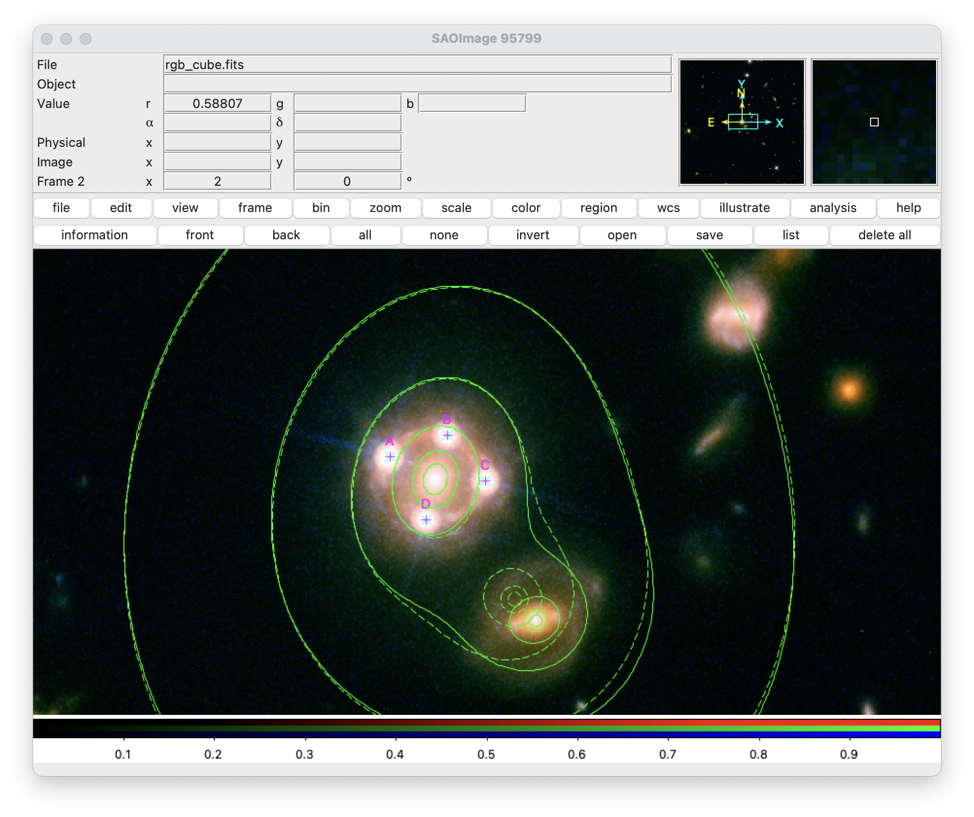
Gravity.plottruelenses! — Method
plottruelenses[!]([backend], model, pars; kw...)Display the true lenses using the given backend or the last backend.
For single-plane lens systems, this routine is identical to plotlenses. However, if there are two or more lensing planes, then this routine plot the true lenses, at the positions one would observe if no gravitational lensing were present. This is generally not what one desires, as the true lens positions and shapes can differ significantly from the observed ones.
The lenses have a size which is proportional to their Einstein radius.
Keywords
filter: if specified, can be used to display a subset of lenses (can be a string interpreted as a globbing pattern, a regular expression, a list, or a function of the lens names)fill: the color used to fill the lenses as a float (indicating a transparency value, by default 0.1) or a tuple (color, transparency)scale: a positive number used to rescale all Einstein radii (default: 0.25)minsize: the minimum size a lens can have, used to display undercritical lenses (default: 0.1)format: The format to use for labels: "%l" is replaced with the lens name and "%z" with the lens redshift (default: "%l" if plotting up to 5 lenses, "" otherwise)
The standard keywords color, linewidth, linestyle, font, fontsize are recognized.
Gravity.plottruemass! — Method
plottruemass[!]([backend,] model, pars; kw...)Plot the true mass distribution of a lensing model.
This function is identical to Gravity.plotmass!, but displays contours associated with the true mass distribution (ignoring all lensing effects).
Intermediate-level routines
Gravity.plotlenses! — Method
plotlenses[!](lenses; kw...)Display a set of lenses using the given backend or the last backend.
The parameter lenses must be a dictionary, created for example with Main.model.flat_lenses. Lenses are shown as contours proportional to their Einstein radii (computed for Dₗₛ / Dₛ = 1).
Keywords
fill: the color used to fill the lenses as a float (indicating a transparency value, by default 0.1) or a tuple (color, transparency)scale: a positive number used to rescale all Einstein radii (default: 0.25)minsize: the minimum size a lens can have, used to display undercritical lenses (default: 0.1)format: The format to use for labels: "%l" is replaced with the lens name and "%z" with the lens redshift (default: "%l" if plotting up to 5 lenses, "" otherwise)
The standard keywords color, linewidth, linestyle, font, fontsize are recognized.
Gravity.plotimages! — Method
plotimages[!]([backend,] images; kw...)Display a set of images using the given backend or the last backend.
The parameter images must be a dictionary, created for example with Main.model.flat_images, Main.model.flat_predictions, or Main.model.flat_sources. Point-like (exact) sources are shown by default with a single cross; image measurement, additionally, can display an ellipse proportional to their covariance matrix.
Keywords
format: the format to use for the image names: can use "%s" and "%i" to represent, respectively, the source and image name, "%m" the image magnitude, and "%t" the image time delay (default: `"%s.%i")scale: a positive number used to rescale all uncertainties (default: 1)minsize: the minimum size an uncertainty can have (default: 0.1)
The standard keywords color, shape (default: :+), size, linewidth, linestyle, font, fontsize are recognized.
Gravity.plotcounterimages — Method
plotcounterimages[!]([backend,] lenssys, z [, x₁, x₂...]; kw...)Display the counter-images associated to one or more images.
This function compute the counter-image position(s) associated to one or more images. For interactive backends, this function can also let the user to choose the image position on the screen. Otherwise, each of the xᵢ must be either a multivariate distribution, or a tuple with the coordinates of the image position. The counter-images are found using Gravity.counterimages.
The parameters z can be a single positive value (the sounrce redshift), or also a range: in that case, a set of counter-images are displayed corresponding to all redshifts in the range. The format keyword can be used to display source details, as
Keywords
scale: a positive number used to rescale all uncertainties (default: 1)minsize: the minimum size an uncertainty can have (default: 0.1)
The standard keywords color, shape (default: :+), size, linewidth, linestyle, font, fontsize are recognized.
Other keywords (grid=:auto, cricticalcurves=3, images=3, lenses=3 are passed to Gravity.counterimages.
Gravity.plotcontours! — Function
plotcontours[!]([backend,] fun, grid; mapping=identity, kw...)Display contours of a function.
This function displays contours of fun, which is taken to be a simple function of the sky posizion x. The function is evaluated at the corners of grid (which must be a Gravity.MaskedGrid), and refinements are possibly computed.
This procedure works in two different modes depending on the value of the keyword levels. If levels is a vector or list of reals, the contours are drawn at the exact values specified. If, instead, levels is a positive integer, suitable levels are found by mapping the function as done by Gravity.plotmap!.
Keywords
levels: a positive integer the number of contours to show, or an array with the exact values of the levels to display (default: 7)refinements: the refinements to compute around the contours (default: 3)mapping: contours can be warped using this function, which must accept an array ofSPoints (useful to display caustic lines)
The keywords zrange, transfer, and logexp are also considered if levels is an integer.
The standard keywords color, linewidth, and linestyle are recognized.
plotcontours[!]([backend,] fun, lenssys, args...; mapping=identity, grid=:auto, kw...)Display contours of a function of a Gravity.LensSystem.
This function displays contours of fun, possibly modified with mapping. fun is taken to accept as arguments fun(lenssys, args..., x). By default contours are displayed on an automatic grid computed using Gravity.lensing_area.
Keywords
grid: AGravity.MaskedGridor:auto(the default), to have the grid automatically computed usingGravity.lensing_arealevels: a positive integer the number of contours to show, or an array with the exact values of the levels to display (default: 7)refinements: the refinements to compute around the contours (default: 3)mapping: contours can be warped using this function, which must accept an array ofSPoints (useful to display caustic lines)
The standard keywords color, linewidth, and linestyle are recognized.
Gravity.plotmap! — Function
plotmap[!]([backend,] fun, grid; mapping=identity, kw...)Display a function as a heatmap.
This function displays fun, which is taken to be a simple function of the sky posizion x. The function is evaluated at the centers of grid (which must be a Gravity.BasicGrid).
This function transforms the values of fun as follows. First, the function is evaluated in the grid and the quantiles specified by the zrange keyword are extracted. The function is then clipped within this range, rescaled in the range [0, 1], and transformed according to the transfer keyword. The resulting values are then displayed.
Keywords
zrange: a single positive number not larger than unity, or a tuple(zmin, zmax)used to select quantiles (default: 0.995)transfer: a symbol representin a standard SAOImage DS9 scale function (:linear,:log,:pow,:sqrt,:square,:asinh,:sinh), or a function (default::sqrt)logexp: a positive number used as a parameter iftransfer=:logortransfer=:pow(default: 1000)
plotmap[!]([backend,] fun, lenssys, args...; grid=:auto, kw...)Display a function of a Gravity.LensSystem.
fun is taken to accept as arguments fun(lenssys, args..., x). Moreover, by default the function is displayed on an automatic grid computed using Gravity.lensing_area.
Gravity.plotgrid! — Method
plotgrid[!]([backend,] grid [, mapped_corners]; kw...)Make a plot of a Gravity.MaskedGrid.
If the optional argument mapped_corners is provided, the plots uses it instead of grid.corners to draw the grid. This is useful to show the effects of a mapping on the grid. The argument must have the same type of grid.corners, i.e. it must be an array of SPoint's.
Keyword parameters
All keywords can be true, false, or a dictionary/named tuple with a set of parameters. They control the grid elements displayed. If set to true, the corresponding element will be shown using pre-determined default attributes. By default, only the grid lines are shown.
grid: the grid itself (solid grey lines)centers: the grid centers (red circles)corners: the grid corners (blue squares)centerlines: the lines connecting nearby corners (light red)cornerlines: the lines connecting a center with its corners (light blue)
Additionally, the centersann, cornersann, centerlinesann, and cornerlinesann keywords control the display of annotation for the relevant grid element. They are all set to false by default.
The keyword levels controls which cell levels are shown: by default all levels are displayed.
Example
julia> using CairoMakie
julia> mask = [1 0; 1 1; 0 1];
julia> grid = Gravity.MaskedGrid(mask, SPoint(0.0, 0.0), SPoint(1.0, 1.0));
julia> Gravity.refine_grid!(grid, [2, 3]);
julia> Gravity.refine_grid!(grid, [7, 8, 9]);
julia> fig = Figure();
julia> ax = Axis(fig[1,1]; aspect=DataAspect(), xgridvisible = false, ygridvisible = false);
julia> Gravity.plotgrid!(ax, grid; centers=true, centersann=true, corners=true);
julia> fig