Gravity
An efficient Bayesian strong gravitational lensing code in Julia.
Features
- Implemented in Julia
- Speed: compiles to native code (using the LLVM technology)
- Interactive
- Good support for parallel and distributed code
- Lensing library
- Highly optimized (micro-benchmarks, automatic differentiation, test units)
- Multi-plane gravitational lensing equations
- Fully Bayesian, with arbitrary prior distributions for all lensing and cosmology parameters
- User-friendly YAML modeling
- Automatic generation of code associated to the model
- Flexible specification of free and linked parameters
- Several techniques to sample the posterior distribution (MH, EMCEE, parallel tempering, HMC, nested sampling...)
- Depending on the sampling technique, can compute the model evidence (with results largely independent of the scheme used)
Acknowledgments
This project has been funded under the National Recovery and Resilience Plan (NRRP), funded by the European Union – NextGenerationEU; Project title “GRAVITY”, project code PNRRBAC24MLOMB01, CUP C53C22000350006
Installation
Direct installation
[Optional] Open a terminal, and check the shell you use with the command
> echo $SHELLIf you use
bashorzshas shell, type> export JULIA_PKG_USE_CLI_GIT=trueOtherwise, if you use
cshortcshtype> setenv JULIA_PKG_USE_CLI_GIT trueThis command, although not strictly necessary, often solves connection issues with GitHub.
Open Julia by entering the command
> julia -t autoWithin the Julia REPL, type
]to enable package mode. There enter the following command(@v1.10) pkg> add https://github.com/astrozot/Gravity.jlIf you have issues with GitHub authentication, you can also use a password-protected SSH key (make sure to have enabled this option in the GitHub repository)
(@v1.10) pkg> add git@github.com:astrozot/Gravity.jl.gitType the
backspaceordeletekey to return to the usual Julia REPL mode. There typejulia> using Gravity
In the future, if you want to use an update version of the package, you can just open Julia, enable the package mode by typing ], and enter
(@v1.10) pkg> updateLocal download or clone
Download code from GitHub and, if necessary, unzip it. Alternatively, clone the package by entering from the shell
> git clone https://github.com/astrozot/Gravity.jlor
> git clone git@github.com:astrozot/Gravity.jl.gitif you use SSH authentication.
Go in the
Gravity.jldirectory and open Julia by entering from the shell> julia --project=. -t autoThis will set the current environment to
Gravityand enable a number of threads (by choosing an appropriate number of threads).Within the Julia REPL, type
]to enable package mode. There enter the following commands(Gravity) pkg> add https://github.com/astrozot/StaticArrays.jl (Gravity) pkg> instantiate (Gravity) pkg> updateType the backspace key to return to the usual Julia REPL mode. There type
julia> using Gravity
If everything proceeds well you should now be ready to use Gravity on a gravitational lensing model.
Examples
Example 1: galaxy-scale system
You can find a few examples of configuration files in the example directory.
As a start, we will consider the galaxy-scale system HE0435-1123: this is composed by a main elliptical galaxy at $z = 0.4546$ that produces four images of a background quasar at $z = 1.689$. A secondary lensing galaxy at $z = 0.7821$ is also included in the model, so this is an example of multi-plane gravitational lensing.
To load the model and perform the inference on the parameters you type the following commands inside the Julia shell:
julia> using Gravity

julia> model = gravitymodel("examples/HE0435-1123/HE0435-1123mag.yml")
Main.GravityModel

julia> chain = runmodel(model)
This will perform a Bayesian inference and, in less than a minute on a typical laptop, display on the screen the final results obtained. You can visualize the distributions obtained for this model using the commands
julia> using CairoMakie, PairPlots

julia> pairplot(chain)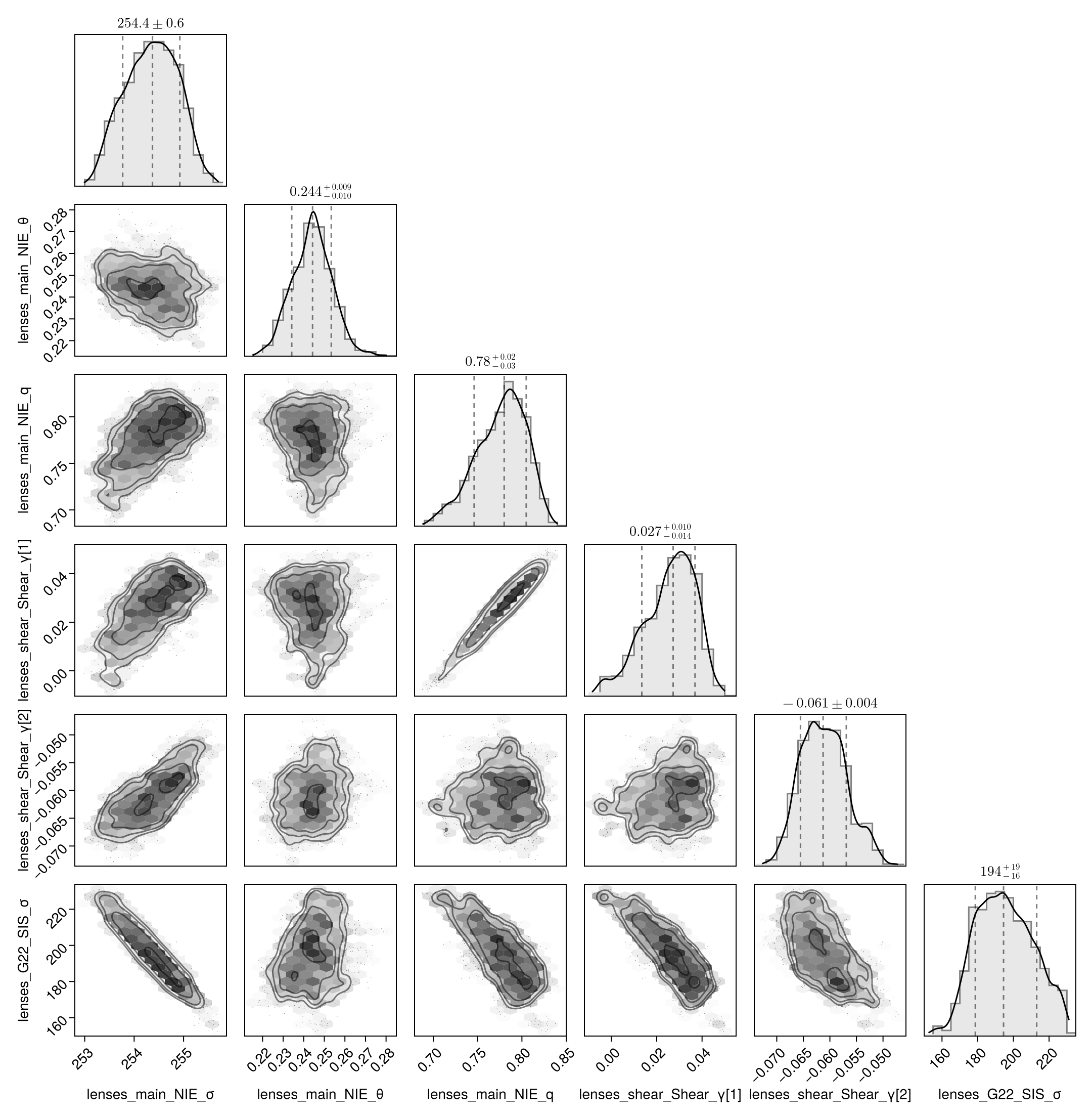
Finally, you can display the best-fit parameters and lensing configuration of the best-fit model with the simple commands
julia> best = bestlp(chain)[2]
6-element Vector{Float64}:
 254.15048135481314
   0.2469213324203622
   0.7707409420002984
   0.02351167383066497
  -0.06197635987278063
 201.50423747216183

julia> plotmodel(model, best; caustics=true, sources=true)
You should see something like the following figure:

Here the blue light-filled shapes indicate the lenses, the green lines are the critical lines computed for the redshift of the source, and the orange asteroids are the corresponding caustic lines. Note how the observed images (pink crosses) are perfectly over-imposed to the predicted ones (cyan x symbols).
Example 2: galaxy cluster RXJ2248
As a second example, we will consider the galaxy cluster RXJ2248 at $z = 0.348$. We model it with two main dark-matter halos, three smooth ellitpical mass distributions representing the intra-cluster gas, and 222 cluster members. The model is based on 55 images divided in 20 families (i.e., originating from 20 sources). In this case, we also perform inference on the cosmological model, and in particular on the $\Omega_\mathrm{m}$ and $w_0$ parameters; we consider a flat cosmology.
julia> using Gravity, CairoMakie, PairPlots

julia> model = gravitymodel("examples/HE0435-1123/HE0435-1123mag.yml")
Main.GravityModel

julia> chain = runmodel(model)
In a few minutes on a modern laptop one will obtain the full parameter inference for this model. A full report of the analysis can be directly obtained with the command
julia> savereport("report", chain)This will create a very detailed report of the whole analysis under the directory ./report.
Citing
If you use Gravity.jl please cite the main reference paper:
For your convenience you can find below the associated BibTeX entry.
@ARTICLE{2024A&A...690A.346L,
       author = {{Lombardi}, Marco},
        title = "{Gravity.jl: Fast and accurate gravitational lens modeling in Julia: I. Point-like and linearized extended sources}",
      journal = {\aap},
     keywords = {gravitational lensing: strong, methods: numerical, methods: statistical, Astrophysics - Instrumentation and Methods for Astrophysics},
         year = 2024,
        month = oct,
       volume = {690},
          eid = {A346},
        pages = {A346},
          doi = {10.1051/0004-6361/202451214},
archivePrefix = {arXiv},
       eprint = {2406.15280},
 primaryClass = {astro-ph.IM},
       adsurl = {https://ui.adsabs.harvard.edu/abs/2024A&A...690A.346L},
}
Outline
- Report on a Gravity.jl execution
- Concrete sources
- Constants
- Cosmology
- Distance coefficients
- GPU acceleration
- Grids
- Gravity
- Lens inversion
- Lens models
- Likelihood
- Luminosity and Mass Profiles
- Lens collections
- Points and related quantities
- Catalogs
- Section
cosmology - Introspection
- Setup
- Section
lens-inversion - Section
lenses - Section
parameters - Pipeline
- Section
sampling - Section
sources - Post processing utilities
- WCS and Data Sections
- Simulations
- Single lenses
- Source Types
- Basic Bayesian techniques
- Image-plane likelihood
- Gravitational lensing theory
- Linear extended sources
- Theory of point-image measurements
- Source-plane likelihood
- Measurement errors
- Utilities
- Visual interface